


Ý tưởng cơ bản của thuật toán Gradient Boosting là lần lượt thêm các decision trees nối tiếp nhau. Tree thêm vào sau sẽ cố gắng giải quyết những sai sót của tree trước đó. Câu hỏi đặt ra là bao nhiêu trees (weak learner hay estimators) là đủ?
Trong bài nãy, hãy cùng nhau tìm hiều cách lựa chọn số lượng và kích thước của các trees phù hợp với từng bài toán của các bạn.
1. Tune số lượng của decision tree
Thông thường khi sử dụng GBM, ta thường chọn số lượng trees tương đối nhỏ. Có thể là vài chục, vài trăm, hoặc vài nghìn. Nguyên nhân có lẽ là vì tăng số lượng trees lên nhiều hơn, hiệu năng của model cũng không tăng, thậm chí còn giảm đi so với khi sử dụng số lượng trees ít hơn.
Mình sẽ sử dụng Otto dataset để minh họa việc tuning số lượng trees. Ở đây mình sử dụng 10-fold cross-validation, số lượng trees trong khoảng [50, 400, 50] -> Có 80 models được train.
Số lượng của trees được chỉ ra bởi giá trị của tham số n_estimators.
# XGBoost on Otto dataset, Tune n_estimators
from pandas import read_csv
from xgboost import XGBClassifier
from sklearn.model_selection import GridSearchCV
from sklearn.model_selection import StratifiedKFold
from sklearn.preprocessing import LabelEncoder
import matplotlib
matplotlib.use('Agg')
from matplotlib import pyplot

# load data
data = read_csv('train.csv')
dataset = data.values

# split data into X and y
X = dataset[:,0:94]
y = dataset[:,94]

# encode string class values as integers
label_encoded_y = LabelEncoder().fit_transform(y)

# grid search
model = XGBClassifier()
n_estimators = range(50, 400, 50)
param_grid = dict(n_estimators=n_estimators)
kfold = StratifiedKFold(n_splits=10, shuffle=True, random_state=7)
grid_search = GridSearchCV(model, param_grid, scoring="accuracy", n_jobs=-1, cv=kfold, verbose=1)
grid_result = grid_search.fit(X, label_encoded_y)

# summarize results
print("Best: %f using %s" % (grid_result.best_score_, grid_result.best_params_))
means = grid_result.cv_results_['mean_test_score']
stds = grid_result.cv_results_['std_test_score']
params = grid_result.cv_results_['params']
for mean, stdev, param in zip(means, stds, params):
    print("%f (%f) with: %r" % (mean, stdev, param))

# plot
pyplot.errorbar(n_estimators, means, yerr=stds)
pyplot.title("XGBoost n_estimators vs accuracy")
pyplot.xlabel('n_estimators')
pyplot.ylabel('accuracy')
pyplot.savefig('_estimators.png')
Kết quả:
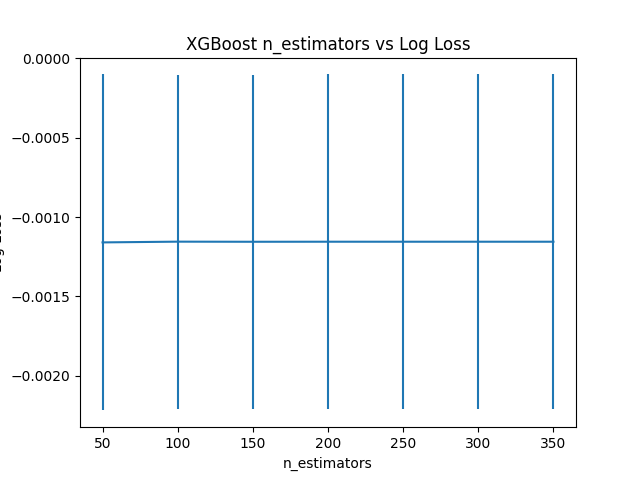
Best: -0.001155 using {'n_estimators': 100}
-0.001160 (0.001059) with: {'n_estimators': 50}
-0.001155 (0.001053) with: {'n_estimators': 100}
-0.001156 (0.001054) with: {'n_estimators': 150}
-0.001155 (0.001054) with: {'n_estimators': 200}
-0.001155 (0.001054) with: {'n_estimators': 250}
-0.001155 (0.001054) with: {'n_estimators': 300}
-0.001155 (0.001054) with: {'n_estimators': 350}
Số lượng trees phù hợp nhất là 100, neg_log_loss đạt được tại đó là -0.001055. Hiệu năng của model không được cải thiện khi tăng số lượng trees từ 100 lên 350.
Đồ thị bên dưới thể hiện mối quan hệ giữa số lượng trees và inverted logarihmic:
2. Tune kích thước của decision tree
Kích thước của tree hay còn gọi là số lớp (layers) hay độ sâu (depth) của tree đó. Nếu tree quá nông (shallow) sẽ dẫn đến underfitting vì model chỉ học được rất ít chi tiết từ dữ liệu. Ngược lại, tree quá sâu (deep) thì model lại học quá nhiều chi tiết từ dữ liệu -> overfitting.
Kích thước của tree được chỉ ra bởi giá trị của tham số max_depth. Ta sẽ thử grid-seach tham số này theo phạm vi [1, 11, 2].
Code đầy đủ như bê dưới:
# XGBoost on Otto dataset, Tune max_depth
from pandas import read_csv
from xgboost import XGBClassifier
from sklearn.model_selection import GridSearchCV
from sklearn.model_selection import StratifiedKFold
from sklearn.preprocessing import LabelEncoder
import matplotlib
matplotlib.use(✬Agg✬)
from matplotlib import pyplot

# load data
data = read_csv('train.csv')
dataset = data.values

# split data into X and y
X = dataset[:,0:94]
y = dataset[:,94]

# encode string class values as integers
label_encoded_y = LabelEncoder().fit_transform(y)

# grid search
model = XGBClassifier()
max_depth = range(1, 11, 2)
print(max_depth)
param_grid = dict(max_depth=max_depth)
kfold = StratifiedKFold(n_splits=10, shuffle=True, random_state=7)
grid_search = GridSearchCV(model, param_grid, scoring="accuracy", n_jobs=-1, cv=kfold, verbose=1)
grid_result = grid_search.fit(X, label_encoded_y)

# summarize results
print("Best: %f using %s" % (grid_result.best_score_, grid_result.best_params_))
means = grid_result.cv_results_['mean_test_score']
stds = grid_result.cv_results_['std_test_score']
params = grid_result.cv_results_['params']
for mean, stdev, param in zip(means, stds, params):
print("%f (%f) with: %r" % (mean, stdev, param))

# plot
pyplot.errorbar(max_depth, means, yerr=stds)
pyplot.title("XGBoost max_depth vs accuracy")
pyplot.xlabel('max_depth')
pyplot.ylabel('accuracy')
pyplot.savefig('max_depth.png')
Kết quả:
Fitting 10 folds for each of 5 candidates, totalling 50 fits
[Parallel(n_jobs=-1)]: Using backend LokyBackend with 12 concurrent workers.
[Parallel(n_jobs=-1)]: Done 26 tasks | elapsed: 5.0min
[Parallel(n_jobs=-1)]: Done 50 out of 50 | elapsed: 7.8min finished
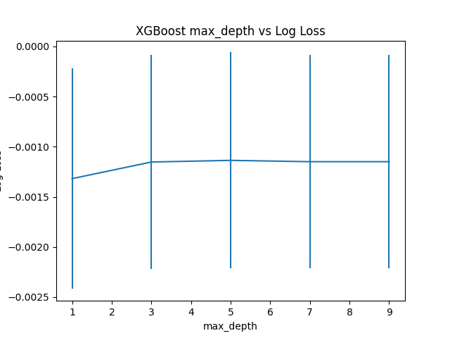
Best: -0.001136 using {'max_depth': 5}
-0.001319 (0.001100) with: {'max_depth': 1}
-0.001153 (0.001066) with: {'max_depth': 3}
-0.001136 (0.001077) with: {'max_depth': 5}
-0.001150 (0.001063) with: {'max_depth': 7}
-0.001150 (0.001063) with: {'max_depth': 9}Quan sát ouput, ta thấy rằng max_depth = 5 cho kết quả tốt nhất. Tăng giá trị này lên 7 hoặc 9, hiệu năng của model không những không được cải thiện mà còn kém đi.
Đồ thị thể hiện mối quan hệ của kích thước tree và neg_log_loss.
3. Tune đồng thời số lượng và kích thước của decision tree
Có một mối liên hệ giữa số lượng và kích thước của mỗi tree. Nhiều tree hơn thì kích thước của mỗi tree sẽ nhỏ hơn. Ngược lại, ít tree hơn thì kích thước của mỗi tree sẽ lớn hơn.
Để tìm ra cặp giá trị (n_estimators, max_depth) phù hợp, ta sẽ thử grid-search như sau:
- n_estimators: (50, 100, 150, 200)
- max_depth: (2, 4, 6, 8)
- 10-fold cross-validation
-> 4x4x10 = 160 models
Code đầy đủ bên dưới:
# XGBoost on Otto dataset, Tune n_estimators and max_depth
from pandas import read_csv
from xgboost import XGBClassifier
from sklearn.model_selection import GridSearchCV
from sklearn.model_selection import StratifiedKFold
from sklearn.preprocessing import LabelEncoder
import matplotlib
matplotlib.use('Agg')
from matplotlib import pyplot
import numpy

# load data
data = read_csv('train.csv')
dataset = data.values

# split data into X and y
X = dataset[:,0:94]
y = dataset[:,94]

# encode string class values as integers
label_encoded_y = LabelEncoder().fit_transform(y)

# grid search
model = XGBClassifier()
n_estimators = [50, 100, 150, 200]
max_depth = [2, 4, 6, 8]
print(max_depth)
param_grid = dict(max_depth=max_depth, n_estimators=n_estimators)
kfold = StratifiedKFold(n_splits=10, shuffle=True, random_state=7)
grid_search = GridSearchCV(model, param_grid, scoring="accuracy", n_jobs=-1, cv=kfold, verbose=1)
grid_result = grid_search.fit(X, label_encoded_y)

# summarize results
print("Best: %f using %s" % (grid_result.best_score_, grid_result.best_params_))
means = grid_result.cv_results_['mean_test_score']
stds = grid_result.cv_results_['std_test_score']
params = grid_result.cv_results_['params']
for mean, stdev, param in zip(means, stds, params):
print("%f (%f) with: %r" % (mean, stdev, param))

# plot results
scores = numpy.array(means).reshape(len(max_depth), len(n_estimators))
for i, value in enumerate(max_depth):
pyplot.plot(n_estimators, scores[i], label='depth: ' + str(value))
pyplot.legend()
pyplot.xlabel('n_estimators')
pyplot.ylabel('accuracy')
pyplot.savefig('n_estimators_vs_max_depth.png')
Kết quả:
Best: -0.001131 using {'max_depth': 4, 'n_estimators': 100}
-0.001266 (0.001112) with: {'max_depth': 2, 'n_estimators': 50}
-0.001249 (0.001101) with: {'max_depth': 2, 'n_estimators': 100}
-0.001248 (0.001101) with: {'max_depth': 2, 'n_estimators': 150}
-0.001247 (0.001100) with: {'max_depth': 2, 'n_estimators': 200}
-0.001141 (0.001094) with: {'max_depth': 4, 'n_estimators': 50}
-0.001131 (0.001088) with: {'max_depth': 4, 'n_estimators': 100}
-0.001132 (0.001089) with: {'max_depth': 4, 'n_estimators': 150}
-0.001132 (0.001089) with: {'max_depth': 4, 'n_estimators': 200}
-0.001160 (0.001059) with: {'max_depth': 6, 'n_estimators': 50}
-0.001155 (0.001053) with: {'max_depth': 6, 'n_estimators': 100}
-0.001156 (0.001054) with: {'max_depth': 6, 'n_estimators': 150}
-0.001155 (0.001054) with: {'max_depth': 6, 'n_estimators': 200}
-0.001155 (0.001068) with: {'max_depth': 8, 'n_estimators': 50}
-0.001150 (0.001063) with: {'max_depth': 8, 'n_estimators': 100}
-0.001150 (0.001064) with: {'max_depth': 8, 'n_estimators': 150}
-0.001150 (0.001064) with: {'max_depth': 8, 'n_estimators': 200}
Từ kết quả ta thấy kết quả tốt nhất đạt được tại max_depth=4 và n_estimators=100, tương tự như kết quả của 2 lần tuning riêng rẽ 2 tham số ở bên trên.
Đồ thị thể hiện mối quan hê của mỗi max_depth với các giá trị của n_estimators.
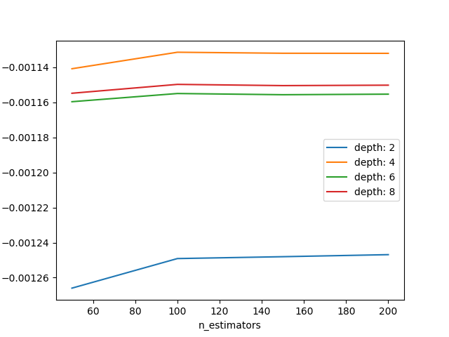
Kết quả thể hiện trên đồ thị cũng minh họa cho nhận định về mối quan hệ giữa số lượng và kích thước của tree mà ta đã nói bên trên.
6. Kết luận
Qua bài viết này, chúng ta đã biết cách tuning XGBoost model, sử dụng phương pháp grid-search (hỗ trợ bởi thư viện scikit-learn) để tìm được số lượng và kích thước của trees phù hợp với bài toán đặt ra ban đầu. Ngoài phương pháp này, còn có 1 phương pháp khác cũng rất hiệu quả là bayes (sử dụng định luật bayes). Phương pháp này thước được các ông lớn AWS, Google, … sử dụng trong các dịch vụ về AI của họ.
Bài viết tiếp theo chúng ta sẽ tiếp tục tune learning_rate đồng thời với số lượng của tree trong XGboost model. Hãy cùng đón đọc! 🙂
Toàn bộ source code của bài này các bạn có thể tham khảo trên github cá nhân của mình tại github.
Xem bài viết gốc tại đây.


Vui lòng đăng nhập để bình luận.