XGBoost – Bài 13: Tuning Learning_Rate và số lượng của Decision Tree

Chào mọi người! Mình là SuNT, đến từ team AI - VTI VN!

Trước đây, mình có ý định viết một chuỗi các bài về XGBoost, một thuật toán rất mạnh mẽ trong Machine Learning (danh sách các bài viết đã public, các bạn có thể xem tại đây). Nhưng thời gian qua, có một số xáo trộn trong công việc nên mình bị gián đoạn, không thể tiếp tục được. Hôm nay mình xin quay lại để hoàn thành nốt ý định đó.

Trong bài này, chúng ta sẽ tìm cách tinh chỉnh (tuning) 2 tham số learning_rate và số lượng trees để nâng cao độ chính xác của XGBoost model. Bởi vì, một vấn đề còn tồn tại của XGBoost là khả năng học trên tập dữ liệu huấn luyện một cách rất nhanh chóng nhưng điều này đôi khi dễ dẫn đến hiện tượng overfitting, mặc dù XGBoost đã sử dụng regularization. Và một cách hiệu quả để điều khiển quá trình học của XGBoost chính là sử dụng learning_rate mà chúng ta sẽ tìm hiểu ngay sau đây.

1. Tuning Learning_Rate

Chúng ta tiếp tục sử dụng Otto dataset trong bài này. Sử dụng giá trị mặc định của số lượng trees là 100, ta sẽ đánh giá sự phù hợp của mỗi giá trị learning_rate trong tập sau: [0.0001, 0.001, 0.01, 0.1, 0.2, 0.3]

Có 6 giá trị của learning_rate, kết hợp với 10-fold cross-validation --> Có 60 models được trained.

Code tuning như sau:

# XGBoost on Otto dataset, Tune learning_rate
from pandas import read_csv
from xgboost import XGBClassifier
from sklearn.model_selection import GridSearchCV
from sklearn.model_selection import StratifiedKFold
from sklearn.preprocessing import LabelEncoder
import matplotlib
matplotlib.use('Agg')
from matplotlib import pyplot

# load data
data = read_csv('train.csv')
dataset = data.values

# split data into X and y
X = dataset[:,0:94]
y = dataset[:,94]

# encode string class values as integers
label_encoded_y = LabelEncoder().fit_transform(y)

# grid search
model = XGBClassifier()
learning_rate = [0.0001, 0.001, 0.01, 0.1, 0.2, 0.3]
param_grid = dict(learning_rate=learning_rate)
kfold = StratifiedKFold(n_splits=10, shuffle=True, random_state=7)
grid_search = GridSearchCV(model, param_grid, scoring="accuracy", n_jobs=-1, cv=kfold, verbose=1)
grid_result = grid_search.fit(X, label_encoded_y)

# summarize results
print("Best: %f using %s" % (grid_result.best_score_, grid_result.best_params_))
means = grid_result.cv_results_['mean_test_score']
stds = grid_result.cv_results_['std_test_score']
params = grid_result.cv_results_['params']
for mean, stdev, param in zip(means, stds, params):
    print("%f (%f) with: %r" % (mean, stdev, param))

# plot
pyplot.errorbar(learning_rate, means, yerr=stds)
pyplot.title("XGBoost learning_rate vs Log Loss")
pyplot.xlabel('learning_rate')
pyplot.ylabel('accuracy')
pyplot.savefig('learning_rate.png')

Kết quả:

Fitting 10 folds for each of 6 candidates, totalling 60 fits
[Parallel(n_jobs=-1)]: Using backend LokyBackend with 12 concurrent workers.
[Parallel(n_jobs=-1)]: Done  26 tasks      | elapsed:  9.1min
[Parallel(n_jobs=-1)]: Done  60 out of  60 | elapsed: 13.8min finished
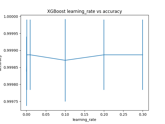
Best: 0.999887 using {'learning_rate': 0.001}
0.999838 (0.000102) with: {'learning_rate': 0.0001}
0.999887 (0.000103) with: {'learning_rate': 0.001}
0.999887 (0.000103) with: {'learning_rate': 0.01}
0.999871 (0.000121) with: {'learning_rate': 0.1}
0.999887 (0.000103) with: {'learning_rate': 0.2}
0.999887 (0.000103) with: {'learning_rate': 0.3}

Giá trị learning_rate tối ưu tìm được là 0.001.

Đồ thị bên dưới thể hiện mối qua hệ giữa learning_rate và độ chính xác của model.

2. Tuning Learning_Rate và số lượng decision tree

Nói chung, khi có nhiều trees được thêm vào XGBoost, những trees thêm vào sau nên sử dụng giá trị learning_rate nhỏ. Ta sẽ kiểm tra nhận định này thông qua quá trình tuning như sau:

• Số lượng trees (n_estimators) = [100, 200, 300, 400, 500]
• learning_rate = [0.0001, 0.001, 0.01, 0.1]

Có 5 giá trị của n_estimators và 4 giá trị của learning_rate, kết hợp với 10-fold cross-validation ta có 200 models cần train.

Code đầy đủ như dưới đây:

# XGBoost on Otto dataset, Tune learning_rate and n_estimators
from pandas import read_csv
from xgboost import XGBClassifier
from sklearn.model_selection import GridSearchCV
from sklearn.model_selection import StratifiedKFold
from sklearn.preprocessing import LabelEncoder
import matplotlib
matplotlib.use('Agg')
from matplotlib import pyplot
import numpy

# load data
data = read_csv('train.csv')
dataset = data.values

# split data into X and y
X = dataset[:,0:94]
y = dataset[:,94]

# encode string class values as integers
label_encoded_y = LabelEncoder().fit_transform(y)

# grid search
model = XGBClassifier()
n_estimators = [100, 200, 300, 400, 500]
learning_rate = [0.0001, 0.001, 0.01, 0.1]
param_grid = dict(learning_rate=learning_rate, n_estimators=n_estimators)
kfold = StratifiedKFold(n_splits=10, shuffle=True, random_state=7)
grid_search = GridSearchCV(model, param_grid, scoring="accuracy", n_jobs=-1, cv=kfold, verbose=1)
grid_result = grid_search.fit(X, label_encoded_y)

# summarize results
print("Best: %f using %s" % (grid_result.best_score_, grid_result.best_params_))
means = grid_result.cv_results_['mean_test_score']
stds = grid_result.cv_results_['std_test_score']
params = grid_result.cv_results_['params']
for mean, stdev, param in zip(means, stds, params):
    print("%f (%f) with: %r" % (mean, stdev, param))

# plot results
scores = numpy.array(means).reshape(len(learning_rate), len(n_estimators))
for i, value in enumerate(learning_rate):
    pyplot.plot(n_estimators, scores[i], label='learning_rate: ' + str(value))
    pyplot.legend()
    pyplot.xlabel('n_estimators')
    pyplot.ylabel('accuracy')
    pyplot.savefig('n_estimators_vs_learning_rate.png')

Sau khoảng 2 tiếng chờ đơi thì chúng ta cũng thu được kết quả:

Fitting 10 folds for each of 20 candidates, totalling 200 fits
[Parallel(n_jobs=-1)]: Using backend LokyBackend with 16 concurrent workers.
[Parallel(n_jobs=-1)]: Done  18 tasks      | elapsed:  6.2min
[Parallel(n_jobs=-1)]: Done 168 tasks      | elapsed: 58.2min
[Parallel(n_jobs=-1)]: Done 200 out of 200 | elapsed: 67.6min finished
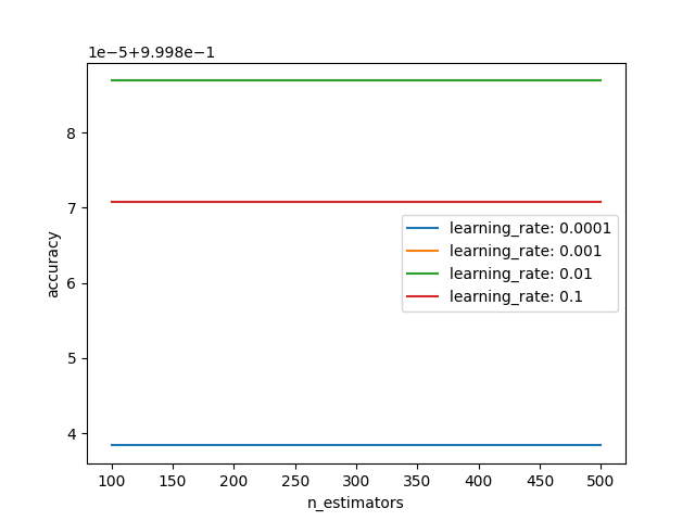
Best: 0.999887 using {'learning_rate': 0.001, 'n_estimators': 100}
0.999838 (0.000102) with: {'learning_rate': 0.0001, 'n_estimators': 100}
0.999838 (0.000102) with: {'learning_rate': 0.0001, 'n_estimators': 200}
0.999838 (0.000102) with: {'learning_rate': 0.0001, 'n_estimators': 300}
0.999838 (0.000102) with: {'learning_rate': 0.0001, 'n_estimators': 400}
0.999838 (0.000102) with: {'learning_rate': 0.0001, 'n_estimators': 500}
0.999887 (0.000103) with: {'learning_rate': 0.001, 'n_estimators': 100}
0.999887 (0.000103) with: {'learning_rate': 0.001, 'n_estimators': 200}
0.999887 (0.000103) with: {'learning_rate': 0.001, 'n_estimators': 300}
0.999887 (0.000103) with: {'learning_rate': 0.001, 'n_estimators': 400}
0.999887 (0.000103) with: {'learning_rate': 0.001, 'n_estimators': 500}
0.999887 (0.000103) with: {'learning_rate': 0.01, 'n_estimators': 100}
0.999887 (0.000103) with: {'learning_rate': 0.01, 'n_estimators': 200}
0.999887 (0.000103) with: {'learning_rate': 0.01, 'n_estimators': 300}
0.999887 (0.000103) with: {'learning_rate': 0.01, 'n_estimators': 400}
0.999887 (0.000103) with: {'learning_rate': 0.01, 'n_estimators': 500}
0.999871 (0.000121) with: {'learning_rate': 0.1, 'n_estimators': 100}
0.999871 (0.000121) with: {'learning_rate': 0.1, 'n_estimators': 200}
0.999871 (0.000121) with: {'learning_rate': 0.1, 'n_estimators': 300}
0.999871 (0.000121) with: {'learning_rate': 0.1, 'n_estimators': 400}
0.999871 (0.000121) with: {'learning_rate': 0.1, 'n_estimators': 500}

Ta có thể thấy, kết quả tốt nhất của model đạt được tại learning_rate=0.001 và n_estimators=100. Tuy nhiên, kết quả này cũng không có sự khác biệt đáng kể so với những trường hợp khác. Bạn có thể thử nghiệm với các metrics đánh giá khác (F1-score, precition, recall, log_loss) để nhìn thấy sự khác biệt rõ hơn.

Bên dưới là đồ thị thể hiện mối quan hệ của mỗi learning_rate với các giá trị khác nhau của n_estimators.

3. Kết luận

Ở bài viết này, chúng ta đã tiến hành tuning XGBoost model với 2 hyper-parameters là learning_rate và n_estimators.

Bài viết tiếp theo chúng ta sẽ tiếp tục tune thêm một tham số khác là subsample. Hãy cùng đón đọc! 🙂

Toàn bộ source code của bài này các bạn có thể tham khảo trên github cá nhân của mình tại github.

Xem bài viết gốc tại đây.